Fill Blank Cells in Excel from Above or Another Sheet
Fill blank cells in Excel with the value above in five steps, or use XLOOKUP to pull missing values from another sheet. Includes formulas and worked examples.
To fill blank cells in Excel, use Go To Special → Blanks for repeated group labels, or a lookup in a helper column when another table contains the missing values. Do not fill unknown amounts with zero: AVERAGE ignores empty cells but includes zeros, so the two produce different results.
For missing department names or regions, fill down from above. For missing prices or employee details, match an ID against a reference sheet. Here are both methods, with examples you can reproduce.
Quick answer
To fill blanks with the value above in Excel for Windows:
- Select the used cells in the label column, including the first known label. Do not select the whole worksheet.
- Press F5 → Special → Blanks → OK.
- Type
=, then press the Up Arrow once to reference the cell above the active blank. - Press Ctrl+Enter to fill all selected blanks with relative formulas.
- Copy the completed range and use Paste Special → Values if the labels must stay fixed when sorting.
Use this for repeated group labels, not unknown costs. The first blank needs a valid label above it; work on an unfiltered copy with clear group boundaries. Cells containing spaces or formulas returning "" are not selected by this method.
Filling from another sheet instead? Use the exact-match XLOOKUP example below. If you need several fields and want the results to follow changing headers, see the dynamic employee lookup with 3,000 source records.
| What the blank represents | Use this method | Check before applying |
|---|---|---|
| A group label omitted on following rows | Go To Special → Blanks, then reference the cell above | The group boundary and the first label are known |
| A value stored in another table | Exact-match lookup in a helper column | Reference keys are unique and source values are complete |
| A value determined by other columns | A formula in a helper column | Inputs are numeric and the business rule is valid |
| A genuinely unknown value | Leave it unresolved and add a status | Do not guess or replace it with zero |
Step 1: Find all missing values
Three quick methods, fastest first:
Go To Special. Select your data range, press F5 → Special… → Blanks → OK. Every blank cell in the range is now selected; give them a fill color so they're visible.
Count them per column:
=COUNTBLANK(B2:B1000)
Filter for them. Add a filter (Ctrl+Shift+L), open a column's dropdown, and check (Blanks) to see exactly which rows are affected.
Also watch for fake blanks: cells containing a space or an empty string "" returned by a formula. COUNTBLANK counts "" but Go To Special → Blanks does not select it. This mismatch is a classic source of confusion:
=SUMPRODUCT(--(TRIM(B2:B1000)=""))
counts true blanks, empty formula results and cells containing only ordinary spaces. It does not remove every invisible character: for example, TRIM alone does not remove a nonbreaking space. See Microsoft's TRIM function guidance before normalizing imported text.
Step 2: Decide what each blank means
This is the step most people skip. A blank can be:
| Meaning | Right action |
|---|---|
| Data exists but wasn't entered | Fill from the source |
| Genuinely zero | Enter 0 explicitly |
| Not applicable | Mark N/A (as text) so it's deliberate |
| Unknown / needs follow-up | Flag it, don't invent a number |
Filling "unknown" with a made-up number is worse than leaving it blank — you've converted visible uncertainty into invisible error.
Step 3: Fill the ones that should be filled
Fill down from above (common for report exports where a category appears once per group): select the range, F5 → Special → Blanks, type = then press the up arrow, and confirm with Ctrl+Enter. Every blank now copies the value above it. Convert to values afterward with Paste Special.
Work on a copy, select only the intended label column, and check that the first blank has a valid label above it. Do not use this method for missing costs or across unrelated groups. Clear filters or explicitly define which rows may change before filling.
Fill-down example with two groups
These are fictional labels. Select only A2:A6, not the entire worksheet column:
| Excel row | Original value in A | Expected value after filling |
|---|---|---|
| 2 | North | North |
| 3 | blank | North |
| 4 | blank | North |
| 5 | South | South |
| 6 | blank | South |
The blank cells A3, A4 and A6 should reference the cell directly above each one. Check that three blanks were filled, both original labels remain and all five rows are still present. After checking, copy A2:A6 and use Paste Special → Values if the labels should stay fixed when you sort the data. Do not extend the selection into empty rows below the dataset.
Compute from other columns. If B holds cost, C revenue and D profit, put this formula in a new helper column E, not in B2. First verify that revenue and profit are valid numbers:
=IF(B2="", C2-D2, B2)
Look it up from another sheet:
=IF(B2="", XLOOKUP(A2, Ref!$A$2:$A$3, Ref!$B$2:$B$3, "CHECK SOURCE"), B2)
Worked example that keeps real zeros
Create a reference sheet named Ref: A2 is A100, B2 is 12, A3 is A200, and B3 is 99. On your working sheet, enter the following inputs in columns A and B. Enter the lookup formula above in E2 and fill down to E4.
| A — Product key | B — Original cost | E — Expected result |
|---|---|---|
| A100 | blank | 12 |
| A200 | 0 | 0 — preserve the original zero |
| A999 | blank | CHECK SOURCE |
The expected outcome is one filled value, one unchanged zero and one unresolved value, not three completed costs. Check that reference keys are unique and reference costs are not blank before using this formula: XLOOKUP returns the first match, and an empty source cost can appear as zero. Review E before pasting approved values into B.
XLOOKUP is not available in Excel 2016 or 2019. In those versions, use an exact-match lookup in the same helper column:
=IF(B2="", IFNA(VLOOKUP(A2, Ref!$A$2:$B$3, 2, FALSE), "CHECK SOURCE"), B2)
For a larger reconciliation example, see matching Excel columns with AI. If a lookup fails unexpectedly, diagnose it with IFNA and XLOOKUP error handling rather than hiding every error.
Step 4: Keep an audit trail
However you fill blanks, record which cells were changed — a highlight color, a "filled" status column, or a change log. Future-you will need to distinguish original data from reconstructed data.
A useful audit table contains:
| Field | Example |
|---|---|
| Row or record key | Order-1042 |
| Column changed | Cost |
| Original value | blank |
| New value | 42.50 |
| Source or rule | Prices!B:B via SKU |
| Review status | Verified |
For large datasets, count missing values before and after by column. A lower blank count is not enough—the number of unresolved and filled values should reconcile to the original total.
Methods to use—and when
- Fill from above: only when blank cells inherit a group label by design.
- Lookup from a reference table: best when a stable key and authoritative source exist.
- Calculate from other fields: safe when the relationship is an accounting or business identity.
- Statistical imputation: appropriate for analysis models, but usually wrong for operational records unless the method is documented.
- Leave blank and flag: correct when the value is genuinely unknown.
If you cannot explain where a filled value came from, do not write it back as fact.
The one-instruction version
With GetSheetAI for Excel open in the sidebar, describe the source, the fill rule and the checks you need:
"Fill the missing costs from the reference sheet by product ID. Keep existing values, including zeros. Put the result on a new sheet and flag anything without a unique, complete source match."
GetSheetAI can help inspect the workbook and write the result back into Excel. Review the changed-cell list and unresolved cases before using the output. If the reference contains several rows per product key, review those duplicate records before trusting a first-match lookup.
Related Excel guidance
Missing values are usually one part of a wider cleanup job. Continue with the complete Excel data-cleaning checklist and review Microsoft's top ways to clean data in Excel.
FAQ
How do I highlight all blank cells in Excel?
Select the range, press F5, choose Special → Blanks, then apply a fill color while they're selected. Conditional formatting with the formula =ISBLANK(A2) keeps future blanks highlighted automatically.
Should missing values be zero or blank?
Only enter 0 when the value is genuinely zero. A blank means "no data," and treating it as zero changes averages and ratios. If a value is unknown, flag it as unknown rather than inventing a number.
Can AI fill missing data in Excel automatically?
AI can help apply a defined fill rule, but it should not invent unknown values. Keep a source copy, request a status and source for each filled cell, and review exceptions before approving the result.